Decoding YOLOv3 output with Intel OpenVINO's backend
Explanation on how the YOLOv3 models output can be decoded from a programming POV
Foreword: The article aims at simplifying the process of getting the understandable results from the RAW output of the YOLOv3 models (v3 and v3-tiny). I will be demonstrating the code snippets from the official demo example provided by OpenVINO toolkit that work for both theses versions but I explain only the v3-tiny which can be generalised for the entire v3 family. Also, I strongly suggest you to get a theoritical understanding of the same from the amazing article by Ethan Yanjia Li. I have almost used Ctrl+C and Ctrl+V from his article to cover up theoritical portions.
Before diving directly into the code, its important to understand some concepts. I will try to summarise them here so they aid in clarifying the other parts.
The YOLOv3 Methodology:
YOLO or You Only Look Once is a single shot detector that is not just another stack of CNNs and FC Layers and perhaps, the paper is itself too chill to give all the crucial details.
Architecture:
The entire system is is divided into two major component: Feature Extractor and Detector, both are multi-scale. When a new image comes in, it goes through the feature extractor first so that we can obtain feature embeddings at three (or more) different scales. Then, these features are feed into three (or more) branches of the detector to get bounding boxes and class information. v3 outputs three feature vectors: (52x52), (26x26) and (13x13) whereas v3-tiny outputs only (26x26) and (13x13).
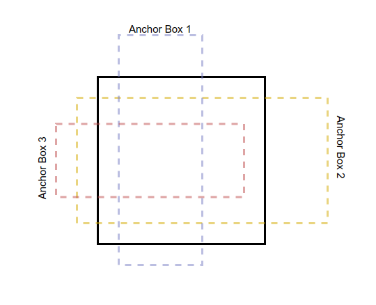
Anchor Box:
This is something very naive yet amazing. It definitely takes some time to sink in. Read this carefully:
The goal of object detection is to get a bounding box and its class. Bounding box usually represents in a normalized xmin, ymin, xmax, ymax format. For example, 0.5 xmin and 0.5 ymin mean the top left corner of the box is in the middle of the image. Intuitively, if we want to get a numeric value like 0.5, we are facing a regression problem. We may as well just have the network predict for values and use Mean Square Error to compare with the ground truth. However, due to the large variance of scale and aspect ratio of boxes, researchers found that it’s really hard for the network to converge if we just use this “brute force” way to get a bounding box. Hence, in Faster-RCNN paper, the idea of an anchor box is proposed.
Anchor box is a prior box that could have different pre-defined aspect ratios (i.e., the authors already have some pre-defined boxes even before the detection begins).
These aspect ratios are determined before training by running K-means on the entire dataset. But where does the box anchor to? We need to introduce a new notion called the grid. In the “ancient” year of 2013, algorithms detect objects by using a window to slide through the entire image and running image classification on each window. However, this is so inefficient that researchers proposed to use Conv net to calculate the whole image all in once.
These aspect ratios or width and height of the anchor boxes are given in the .confg files by the authors. They are not normalised unlike most other values. They are arranged as pair of width and height (w1,h1,w2,h2,w3,h3,…w18,h18) as: pair x 3 anchors x 2 Detector_layers = 18 anchor points (or 9 pairs).
And specifically this last part:
Since the convolution outputs a square matrix of feature values (like 13x13, 26x26, and 52x52 in YOLO), we define this matrix as a “grid” and assign anchor boxes to each cell of the grid. In other words, anchor boxes anchor to the grid cells, and they share the same centroid.
In other words, the authors thought: “Instead of predicting the boxes (or rather their location & dimensions) from scratch, lets place some pre-determined boxes, in the regions where objects are probably found (found using K-Means) and then, the ground-truth (or actual) values (of location and dimensions) for these boxes can be calculated by simply finding the offsets to the location and dimensions of the box”
The two detectors will each be giving a grid of shape:
| Layer/Detector | Grid shape |
|---|---|
| Conv_12 | 26x26 |
| Conv_9 | 13x13 |
Note: We are specifically talking about YOLOv3-tiny. For the larger YOLOv3, another detector gives a grid of shape 52x52. Both these models accept strictly resized images of shape 416x416x3.
If this was image:
Then the grid over the image, by the Conv_9 layer would be
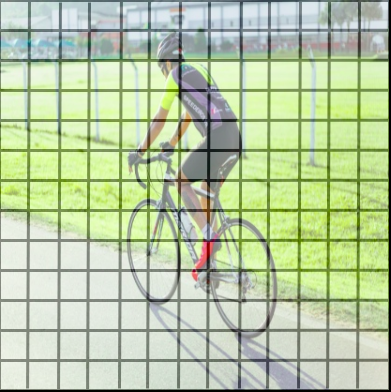
Notice that this also implies that within each cell of a grid, objects are detected using these anchors; that is, the maximum number of objects that can be detected within a cell = number of anchor boxes in it. In v3-tiny, each cell has only 3 anchor boxes. So, each grid cell looks somewhat like this:
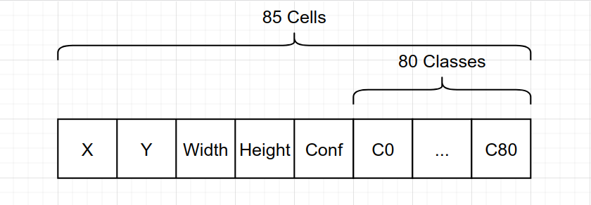
What does each cell hold ?
Each cell has 3 anchors in v3 and v3-tiny. Each anchor has the following attributes of its location, dimensions, objectness score and class probablities:
tx: (a single float) x-coordinate of the centroid (of anchor box) relative to the top-left corner of that cellty: (a single float) y-coordinate of the centroid (of anchor box) relative to the top-left corner of that celltw: (a single float) absolute width of the bounding boxth: (a single float) absolute height of the bounding boxconfidence: (a single float) The probablity that the anchor box did detect some object.class scores: (80 float values) The 80 classes with their scores. If theconfidenceis above our preset threshold, we pick the one class out of these 80 classes, with highest value. The result array looks like
Note: I have used x and y instead of tx and ty in the code and the diagrams. Pardon me for that as I am bound to copy-paste while following the demo code from OpenVINO demos.
To explain tx and ty, for example, tx = 0.5 and ty = 0.5 means the top left corner of the box is in the middle of the image i.e, the centroid of the detected bounding box is at the exact center of that grid cell and not the entire image. Notice that all three anchor boxes of each cell share a common centroid. The absolute value of these bounding boxes has to be calculated by adding the grid cell location (or its index) to its x and y coordinates. To understand, look at the below figure from the official paper and the example below:
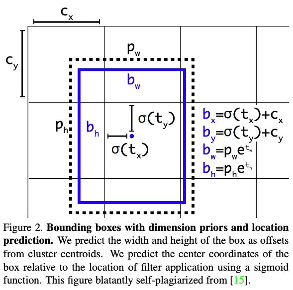
As an example,
(In the figure,) Cx and Cy represents the absolute location of the top-left corner of the current grid cell. So if the grid cell is the one in the SECOND row and SECOND column of a grid 13x13, then Cx = 1 and Cy = 1. And if we add this grid cell location with relative centroid location, we will have the absolute centroid location bx = 0.5 + 1 and by = 0.5 + 1. Certainly, the author won’t bother to tell you that you also need to normalize this by dividing by the grid size, so the true bx would be 1.5/13 = 0.115
tw and th are normalised too. To get absolute values of width and height, we need to multiply them with their respective anchor width or height and again normalize by the image width or height respectively (fixed to 416x416 for v3 and v3-tiny). But why is it so twisted 😕. To that… Its like that
A simplified instruction is:
- Get the normalised
twandthfrom the detections. - Process this value using the exponent or
expfunction. (As we may get -ve or big values sometimes) - Multiply this value with the pre-determined absolute values (aspect ratio) of the anchor box.
- Again normalise this result using aspect ratio of the resized image(416x416).
- Use these results as offsets to get x & y coordinates from the coordinates of the centroid with respect to the center of the bounding box.
The code section below will give you more clarity on it.
What about the code ?
Note: It is assumed that the reader accepts that I have used OpenVINO backend just as any other method to fetch results from the model and only aim to focus the decoding part, which is common.
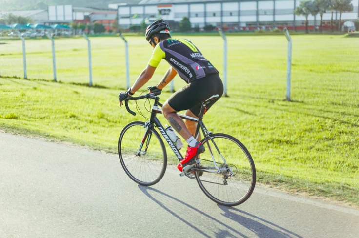
We start with the pre-processed frame pframe fed to the inference engine ie. I use the object infer_network of the class Network. Our original image was:
The pre-processing was done as:
### Pre-process the image as needed ###
     b, c, h, w = infer_network.get_input_shape()
     pframe = cv2.resize(frame,(w,h))
     pframe = pframe.transpose((2,0,1))
     pframe = pframe.reshape((b,c,h,w))
Let’s jump directly into the raw output of the inference.
The output is obtained as output = self.exec_net.requests[0].outputs. This is a dictionary with 2x{Layer, feature_map_values}.
for layer_name, out_blob in output.items():
    print(out_blob.shape)
    print("Layer:{}\nOutBlob:{}".format(layer_name, out_blob))

#Layer                                              |  Feature map shape
#detector/yolo-v3-tiny/Conv_12/BiasAdd/YoloRegion   |   (1, 255, 26, 26)
#detector/yolo-v3-tiny/Conv_9/BiasAdd/YoloRegion    |   (1, 255, 13, 13)
Wait, first Tell me something about the model
Originally, YOLOv3 model includes feature extractor called Darknet-53 with three branches for v3 (and 2 branches for v3-tiny) at the end that make detections at three different scales. These branches must end with the YOLO Region layer. (named as simply YOLO) Region layer was first introduced in the DarkNet framework. Other frameworks, including TensorFlow, do not have the Region implemented as a single layer, so every author of public YOLOv3 model creates it using simple layers. This badly affects performance. For this reason, the main idea of YOLOv3 model conversion to IR is to cut off these custom Region-like parts of the model and complete the model with the Region layers where required. Source
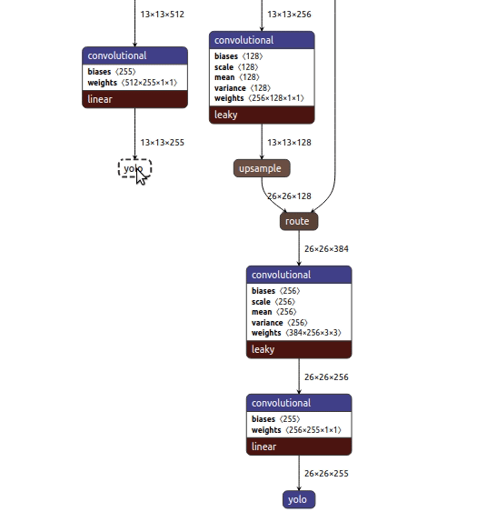
From the above diagram, it seems lucid why we obtained these two layers as output from the Inference Engine. Pre-conversion to IR, they are named as simply YOLO layers while post-conversion, they are named as YoloRegion.
Now, we know that we have 2 layers from v3-tiny. From the theory of anchors and grid, we know that both these layers function differently. So, we start with first finding their parameters. The yolov3-tiny.cfg is the source of all these parameters. We just need to pick them from this file manually OR use the .xml and .bin. We have already initialised the net as:
# Read the IR as a IENetwork
self.net = IENetwork(model = model_xml, weights = model_bin)
These params are extracted from this net as self.net.layers[layer_name].params. In the demo provided by OpenVINO docs, these params or parameters are hard coded as:
class YoloParams:
    # ------------------------------------------- Extracting layer parameters ------------------------------------------
    # Magic numbers are copied from yolov3-tiny.cfg file (Look in the project folder). If the params can't be extracted automatically, use these hard-coded values.
    def __init__(self, param, side):
        self.num = 3 if 'num' not in param else int(param['num'])
        self.coords = 4 if 'coords' not in param else int(param['coords'])
        self.classes = 80 if 'classes' not in param else int(param['classes'])
        self.anchors = [10.0, 13.0, 16.0, 30.0, 33.0, 23.0, 30.0, 61.0, 62.0, 45.0, 59.0, 119.0, 116.0, 90.0, 156.0,
                        198.0,
                        373.0, 326.0] if 'anchors' not in param else [float(a) for a in param['anchors'].split(',')]

        if 'mask' in param:
            mask = [int(idx) for idx in param['mask'].split(',')]
            self.num = len(mask)

            # Collect pairs of anchors to mask/use
            maskedAnchors = []
            for idx in mask:
                maskedAnchors += [self.anchors[idx * 2], self.anchors[idx * 2 + 1]]
            self.anchors = maskedAnchors

        self.side = side    # 26 for first layer and 13 for second
        self.isYoloV3 = 'mask' in param  # Weak way to determine but the only one.

        def log_params(self):
            params_to_print = {'classes': self.classes, 'num': self.num, 'coords': self.coords, 'anchors': self.anchors}
            [log.info("         {:8}: {}".format(param_name, param)) for param_name, param in params_to_print.items()]
To understand the mask mentioned here, actually, the .cfg file provides 6 pairs of anchors. These anchors are divided among these 2 feature (output) layers in a pre-determined fashion; the parameter param stores this info. To look into the param attribute of both these feature layers:
# Layer 1
Params: {'anchors': '10,14,23,27,37,58,81,82,135,169,344,319', 'axis': '1', 'classes': '80', 'coords': '4', 'do_softmax': '0', 'end_axis': '3', 'mask': '0,1,2', 'num': '6'}

# Layer 2
Params: {'anchors': '10,14,23,27,37,58,81,82,135,169,344,319', 'axis': '1', 'classes': '80', 'coords': '4', 'do_softmax': '0', 'end_axis': '3', 'mask': '3,4,5', 'num': '6'}
The attribute mask helps in distributing/allocating the anchors between the layers. Post-process params or the objects of the class YoloParamslook like:
# Layer 1
[ INFO ] Layer detector/yolo-v3-tiny/Conv_12/BiasAdd/YoloRegion parameters:
[ INFO ]          classes : 80
[ INFO ]          num     : 3
[ INFO ]          coords  : 4
[ INFO ]          anchors : [10.0, 14.0, 23.0, 27.0, 37.0, 58.0]

# Layer 2
[ INFO ] Layer detector/yolo-v3-tiny/Conv_9/BiasAdd/YoloRegion parameters:
[ INFO ]          classes : 80
[ INFO ]          num     : 3
[ INFO ]          coords  : 4
[ INFO ]          anchors : [81.0, 82.0, 135.0, 169.0, 344.0, 319.0]
This log is dumped by log_params in the above class. Another important element in the class definition is self.isYoloV3 = 'mask' in param. This simply helps us to determine whether the model being used is v3 or not. Actually, the mask is exclusive to YOLOv3 and tiny version. Previous versions lack it.
After the output layer has been extracted, we have a 3D array filled with mysteriously packed data that is the treasure we seek. The method used to pack has been discussed in the theory part above. We write a parser function that parses/simplifies this and call it parse_yolo_region(). This function takes in the array full of raw values (let’s call it packed array) and gives out list of all detected objects. The function does the following. The two output blobs are (1,255,26,26) and (1,255,13,13). Let it be (1,255,side,side) for this blog (the side attribute is dedicated for this. Look up the definition of the YoloParams class). The side x side represents the grid and the 255 values are the array we showed earlier.
One method to decode this array for both the layers is:
     for oth in range(0, blob.shape[1], 85):   # 255
        for row in range(blob.shape[2]):       # 13
            for col in range(blob.shape[3]):   # 13
                info_per_anchor = blob[0, oth:oth+85, row, col] #print("prob"+str(prob))
                x, y, width, height, prob = info_per_anchor[:5]
Next, we find if any of the anchor boxes found an object and if it did, what class was it. There were 80 classes and the one with the highest probablity is the answer.
if(prob < threshold):
    continue

# Now the remaining terms (l+5:l+85) are 80 Classes
class_id = np.argmax(info_per_anchor[5:])
At the threshold confidence of 0.1 or 10%, the classes detected in our test image of the cycle+man, are
person 	 prob:0.19843937456607819
person 	 prob:0.7788506746292114
bicycle  prob:0.8749380707740784
bicycle  prob:0.8752843737602234
The x and y coordinates obtained are relative to the cell. To get the coordinates with respect to the entire image, we add the grid index and finally normalize the result with the side parameter.
x = (col + x) / params.side
y = (row + y) / params.side
To relate with above explained example, the commands can be related with the following terms used in the original paper.
bx = (Cx + x) / params.side
by = (Cy + y) / params.side
The aspect ratio or width and height, can be a big number or even negative, so we use exponent to correct it.
try:
    width = exp(width)
    height = exp(height)
except OverflowError:
    continue
These values are already normalised. To get absolute values of width and height, we need to multiply them with their respective anchor width or height and again normalize by the image width or height respectively (fixed to 416x416 for v3 and v3-tiny). Why we do this, wait for it…
size_normalizer = (resized_image_w, resized_image_h) if params.isYoloV3 else (params.side, params.side)
n = int(oth/85)
width = width * params.anchors[2 * n] / size_normalizer[0]
height = height * params.anchors[2 * n + 1] / size_normalizer[1]
To similarly get absolute coordinates of top-left and bottom right point of the box, we use the xand y values we determined and use the normalised width and height to get the values. w/2 shifts the point from center of the cell to the left boundary and y/2 shifts it to the upper boundary. Together, they give the top-left corner of the box. To resize these bounding boxes to the original image, we scale it up using the dimensions of the image (w_scale=h_scale=416).
xmin = int((x - w / 2) * w_scale)
ymin = int((y - h / 2) * h_scale)
xmax = int(xmin + w * w_scale)
ymax = int(ymin + h * h_scale)
Now, we have the desired observations from the 2 detector layers and we enpack them into objects to get:
In Layer detector/yolo-v3-tiny/Conv_12/BiasAdd/YoloRegion
Detected Objects
{'xmin': 707, 'xmax': 721, 'ymin': 53, 'ymax': 68, 'class_id': 8, 'confidence': 0.0016403508}


In Layer detector/yolo-v3-tiny/Conv_9/BiasAdd/YoloRegion
Detected Objects
{'xmin': 707, 'xmax': 721, 'ymin': 53, 'ymax': 68, 'class_id': 8, 'confidence': 0.0016403508}
{'xmin': 257, 'xmax': 454, 'ymin': 32, 'ymax': 323, 'class_id': 0, 'confidence': 0.29021382}
{'xmin': 247, 'xmax': 470, 'ymin': 31, 'ymax': 373, 'class_id': 0, 'confidence': 0.34315744}
{'xmin': 231, 'xmax': 534, 'ymin': 165, 'ymax': 410, 'class_id': 1, 'confidence': 0.6760541}
{'xmin': 232, 'xmax': 540, 'ymin': 188, 'ymax': 428, 'class_id': 1, 'confidence': 0.23595412}
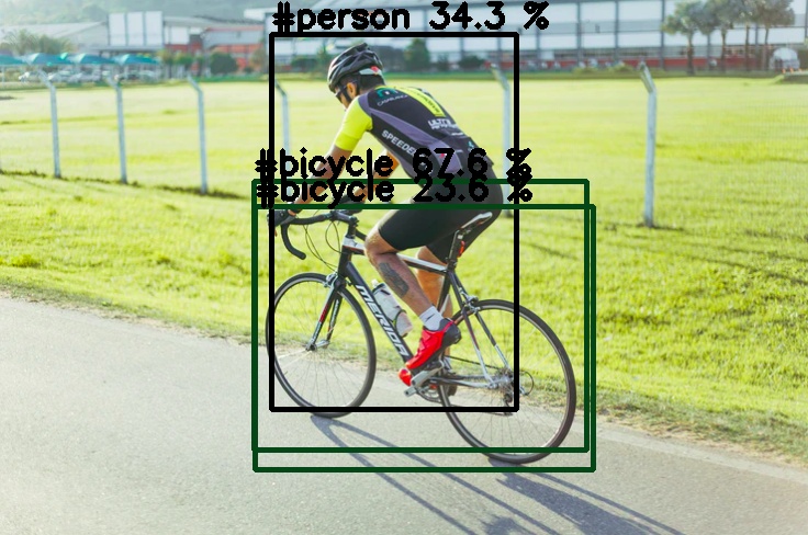
But there are too many detections for just a single bicycle and person; this is an inherent issue with YOLO which leads to duplicate predictions beacause it is very likely that two or more anchors of same or different cell detect a particular object with different or even same probablities. If we plot all these boxes on the image, we get
To remove these duplicate boxes, we employ Non-Maximal Suppression and Intersection over Union.
Non-Maximal Suppression:
Let’s not be perplexed with the fancy term. It would have been just fine even if one didn’t know it; we are already familiar with it but not the name. It refers to filtering objects on the basis of confidence.
Intersection over Union (IoU):
If we have two bounding boxes, then, IoU is defined as
![IoU = dividing the area of overlap between the bounding boxes by the area of union [source]](/img/yolov3_decoding/iou_equation.png)
IoU = dividing the area of overlap between the bounding boxes by the area of union [source]
It is used for two purposes:
- It helps us benchmark the accuracy of our model predictions. Using it, we can figure out how well does our predicted bounding box overlap with the ground truth bounding box. The higher the IoU, the better the performance. The results can be interpreted as
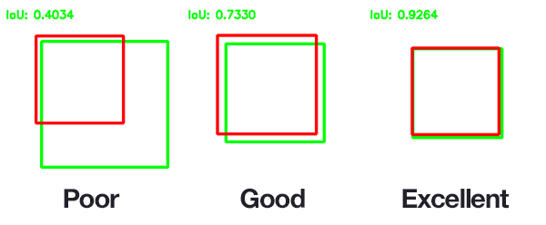
IoU for performance check
- It helps us remove duplicate bounding boxes for the same object. Exactly the problem that we are facing with the cyclist test case. For, this, we sort all the predictions/objects in descending order of their confidence. If two bounding boxes are pointing to the same object, their IoU would definitely be very high. In this case, we choose the box with higher confidence (i.e., the first box) and reject the second one. If the IoU is very low, this would possibly mean that the two boxes point to different objects of the same class(like different dogs or different cats in the same picture). We use IoU solely for this purpose.
    objects = sorted(objects, key=lambda obj : obj['confidence'], reverse=True)

    for i in range(len(objects)):
        if objects[i]['confidence'] == 0:
            continue
        for j in range(i + 1, len(objects)):
            # We perform IOU on objects of same class only
            if(objects[i]['class_id'] != objects[j]['class_id']): continue

            if intersection_over_union(objects[i], objects[j]) > args.iou_threshold:
                objects[j]['confidence'] = 0

    # Drawing objects with respect to the --prob_threshold CLI parameter
    objects = [obj for obj in objects if obj['confidence'] >= args.prob_threshold]
    print(f"final objects:{objects}")
where intersection_over_union is defined as
def intersection_over_union(box_1, box_2):
    width_of_overlap_area = min(box_1['xmax'], box_2['xmax']) - max(box_1['xmin'], box_2['xmin'])
    height_of_overlap_area = min(box_1['ymax'], box_2['ymax']) - max(box_1['ymin'], box_2['ymin'])
    if width_of_overlap_area < 0 or height_of_overlap_area < 0:
        area_of_overlap = 0
    else:
        area_of_overlap = width_of_overlap_area * height_of_overlap_area
    box_1_area = (box_1['ymax'] - box_1['ymin']) * (box_1['xmax'] - box_1['xmin'])
    box_2_area = (box_2['ymax'] - box_2['ymin']) * (box_2['xmax'] - box_2['xmin'])
    area_of_union = box_1_area + box_2_area - area_of_overlap
    if area_of_union == 0:
        return 0
    return area_of_overlap / area_of_union
Post this, we get filtered objects as
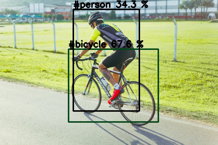
final objects:[{'xmin': 231, 'xmax': 534, 'ymin': 165, 'ymax': 410, 'class_id': 1, 'confidence': 0.6760541}, {'xmin': 247, 'xmax': 470, 'ymin': 31, 'ymax': 373, 'class_id': 0, 'confidence': 0.34315744}]
Now, we have good detections; on drawing bounding boxes, we get the following results at the confidence threshold of 0.1 (10%) and IoU threshold of 0.4 (40%):
The entire code used here can be found in my GitHub Repo [HERE]. But I also suggest you look into the demo provided by Intel (Link in references).
I hope this article made sense. Feel free to find discrepencies in the material, I will try my best to correct them and clarify any doubts in it.
Sources
- OpenVINO YOLO Demo: https://github.com/opencv/open_model_zoo/tree/master/demos/python_demos/object_detection_demo_yolov3_async
- Cyclist Image Used: https://unsplash.com/photos/Tzz4XrrdPUE
- Understanding YOLO : https://towardsdatascience.com/dive-really-deep-into-yolo-v3-a-beginners-guide-9e3d2666280e